How to get the best out of online weather sources, and how far they can be pushed.
Habebant quoque Switenses in manibus quedam instrumenta occisionis gesa, in vulgari illo appellata helnbartam, valde terribilia, quibus adversarios firmissime armatos quasi cum novacula diviserunt et in frusta conciderunt.
The men of Schwyz also had in their hands certain killing tools, glaives, called in their own tongue helnbartam, most terrible, with which they cut even the best-armoured enemy apart as with a razor and hacked him to pieces.
— John of Winterthur, Franciscan friar, on the battle of Morgarten (written in the 1340s)
It started, as Swiss history so often does, with a quarrel over pasture. The cattle farmers of Schwyz and the monks of Einsiedeln had been clearing the same forest from opposite ends for two hundred years, and on the night of Epiphany 1314 the farmers settled the boundary question their own way: they raided the abbey, emptied the wine cellar, and marched the monks home as hostages. The abbey’s schoolmaster wrote it up with feeling: drunk beyond all reason, with “the flame of the devil” driving them on. The abbey stood under the protection of the Habsburgs, a Habsburg was claiming the crown of the Empire, and Schwyz had backed the other candidate. So in November 1315 Duke Leopold of Austria came up the valley to teach a lesson to “those peasants walled in by mountains instead of walls”. John of Winterthur gives him 20,000 men (historians settle for 2,000 or 3,000) and says they were so sure of victory that they brought ropes to lead away the cattle.
On 15 November the column of knights rode along Lake Ägeri, a narrow strip between the steep slope and the water, the kind of road no cavalry commander should take twice. A knight of 1315 was the tank of his day: armoured in mail from head to knee, on a horse that cost as much as a farm, trained since boyhood, and on open ground nothing on foot could stop him. On a lakeshore track, with no room to charge or turn, he was a tank in a ditch. The men of Schwyz were waiting on the slope. Rocks and tree trunks came down first, if later tradition is right; then the farmers themselves, onto the knights “like onto fish caught in a drag-net”. The helnbarten, the first anti-tank weapon a farmer could forge, did the rest: a heavy cleaver blade on a two-metre shaft that split helmets, cut through mail and dragged riders out of the saddle. John again: “there was not a battle, but a slaughter, like a herd led to the shambles”. No prisoners were taken. Whoever could still move fled into the lake, and many drowned in it. Leopold got away with a guide who knew the paths. Three weeks later, at Brunnen, Uri, Schwyz and Unterwalden renewed their alliance, for the first time in German: no lord would be accepted by one without the consent of all.
From there the Swiss built a national legend: the small republic of free farmers against the great princes, and the princes kept supplying the material. Another Duke Leopold of Austria, nephew of the first, rode against the Confederates at Sempach in 1386 and did not ride home. Charles the Bold of Burgundy, the richest prince of his day, lost his treasure at Grandson, his army at Murten and his life at Nancy, in 1476 and 1477 (“at Grandson the goods, at Murten the courage, at Nancy the blood”, as Swiss schoolchildren still learn it). In 1499 the Emperor’s own army was beaten at Calven and Dornach, and the Confederation quietly stopped behaving as part of the Empire. When the next great power came, revolutionary France in 1798, the men of Schwyz under Alois von Reding threw the French back at Rothenthurm and, once again, on the heights of Morgarten. They capitulated two days later anyway, but the symbolism was impeccable. (In fairness to the knights of 1315: most of them came from Lucerne, Zug, Zürich and the Aargau, all of which later joined the winning side. The farmers’ democracy was a meeting of cattle owners in a meadow. A legend doesn’t have to be a seminar.)
What survived all of it is the militia. Swiss soldiers still take their rifles home, shoot a compulsory programme at 300 m every year in a local club, and on one weekend in spring some 110,000 people join them in the Federal Field Shoot, which bills itself, without visible irony, as the largest shooting festival in the world. And every 15 November since 1912, more than a thousand marksmen from all over the country gather at Morgarten, groups of ten, service rifles only, the K31 among them, to shoot at the battle site. The distance is 300 m.
Which is a problem, if you think about it. 300 m is helnbarten range compared with what a K31 can do, and a new enemy will have read the chronicles. He won’t ride along the lakeshore into the farmers’ arms; he will stop at a polite 800 m. So let’s imagine a marksman, and call him Reto. On Sunday he shot the Morgarten shoot with his grandfather’s K31. Now let’s imagine that on Wednesday the new enemy comes up the valley, as Leopold did, and Reto has to face him: lying on the slope above the lake at 730 m above sea level, the enemy at 800 m, a ballistic calculator in his pocket and no weather meter. Before the first shot he takes the pressure off the weather app on his phone, 1000 hPa, and types it into the calculator with the rest: 10 °C, 66 % humidity. The real pressure at 730 m that morning was 916 hPa. His calculator now believes the air is 9 % denser than it is, asks for 0.43 mrad too much at 800 m, and his first shots go about 35 cm high.
Reto does what any of us would do. He trues. The calculator offers to fix the BC of his GP11 from 0.274 to 0.299, or the muzzle velocity from 780 to 797 m/s. He takes the velocity, because “a BC printed on a box can’t be 9 % off”. From then on his 800 m dope is right, his 1000 m dope is 0.2 mrad off when the enemy starts backing away, and the next time he types in a correct pressure he is 0.4 mrad low at 800 m and blames the ammunition lot. (Truing has its own post on this site, “Least Squares, Most Hits“. It can only correct what it is told about.) John of Winterthur’s farmers had the advantage of fighting at arm’s length.
bc.geladen.ch can now fetch the weather for you, from official weather stations nearby. That sounds like a ten-minute job. It wasn’t. This post is the list of things that went wrong on the way, what I did about each, and what each fix was worth, measured on a year of real data. Along the way you’ll see where the weather on your phone and most weather websites go wrong, so you can spot the traps whatever source you use.
While Reto is imaginary, the weather is the app’s real Morgarten fetch of 18 November 2026, 11:29 (9.9 °C, 916.1 hPa, 66 %; airports’ QNH 999–1000 hPa); come-up figures computed with the app’s engine for K31 + GP11.
Reto’s slope isn’t only a figure of speech, by the way. Until you set a position of your own, the app’s default position is the Morgarten battle site, 47.107 °N 8.642 °E, altitude 730 m, in memory of a November morning more than 700 years ago. Press “Get weather” on a fresh install and you get the farmers’ weather.
TL;DR (for the attention-challenged)
- Weather apps and websites mostly show model output and sea-level pressure. Neither belongs in a ballistic calculator.
- What you need is measured air at your height, now. No single weather station gives you that.
- The app combines up to 8 official stations, moves their readings to your height and to the present moment (allowing for clouds), throws out the odd one, and weighs the rest by their distance and by how they are spread around you.
- Result: about 0.6 % typical error in air density, against about 0.8 % for the nearest airport alone. With GP11 that is just under 0.03 mrad at 800 m. A Kestrel used properly is 3 to 5 times better. In the sun, it isn’t.
- Your biggest lever is the height you type in. Read it off a map.
- Don’t true away a weather error. The BC you “fix” at one range is wrong at the next.
Disclaimers
I am not a meteorologist. The data belong to the weather services; my part was choosing, combining and checking them, with an AI doing a good share of the scripting and the arithmetic. The numbers come from a year of real measurements, not from the AI.
Every accuracy figure below is a statistic (§2). It tells you how the app usually does, not how badly it can do, and certainly not what it will do at your firing point.
A handheld weather meter, used properly, still wins (§17). The online weather is for when you don’t have one, or for checking the one you have.
Part I: The target and the yardstick
1. What we are after: air density
Your calculator wants one thing from the weather: air density. Temperature, pressure and humidity are only the ingredients, and they don’t count equally. Here is what one unit of error in each does to density, and to the come-up of a K31 with GP11 from the app’s library (G7 BC 0.274, 780 m/s, 70 mm sight height, 100 m zero, in air of 10 °C at 730 m), in mrad:
| Error of | Air density | mrad at 600 / 800 / 1000 m |
|---|---|---|
| 1 °C | 0.37 % | 0.006 / 0.014 / 0.027 |
| 1 °C, with the powder temperature taken as the air temperature (GP11: 0.8 m/s per °C) | 0.37 % | 0.020 / 0.035 / 0.059 |
| 1 hPa | 0.11 % | 0.002 / 0.005 / 0.010 |
| 10 % relative humidity | 0.05 % | 0.001 / 0.002 / 0.005 |
So 1 °C does as much as 3.4 hPa. And if your calculator uses the air temperature for the powder temperature, as most do when you give them a temperature sensitivity, every degree you get wrong costs twice: once in the air, once in the muzzle velocity.
A word on the temperature rows. The first one is net: warmer air also raises the speed of sound, and near Mach 1 the extra drag gives part of the effect back (A.1). The second row applies only if your calculator takes the powder temperature from the air temperature: GP11 gains about 0.8 m/s per °C, which costs as much as the air itself. The real temperature of the cartridge is another matter: rounds lying on a mat in the sun, or sitting in a hot chamber, are not at air temperature, and no weather station knows about them. The 0.8 m/s per °C is the library’s figure for GP11; your lot may differ.
Everywhere else in this post, an error in mrad means the density error alone, as if it came from pressure: per 1 % of density, 0.021 / 0.047 / 0.094 mrad at 600 / 800 / 1000 m. When the error comes from temperature, the speed of sound takes about a sixth off that; a calculator that ties the powder to the air temperature doubles it at 800 m (1.7 times at 1000 m).
In practice temperature is about 90 % of what goes wrong with weather from stations. Spend your worry on temperature. Humidity can have the leftovers.
2. How each fix was scored
Every “better” and “worse” in Part II comes from one test, and the trick is simple and slightly cruel. Take a station, hide its own report from it, make the app guess its weather from the neighbours within 150 km, then check the answer. Do that for about 5,400 airports and other official stations, every hour of 2025: some 58 million little exams. Reports reach the app as late as they would live, and nothing older than 90 minutes counts. The score is the typical (RMS) error in air density, and a fix stays in only if that number goes down. I kept 2024 back as a second check; it played no part in choosing any setting. A.10 has the gory details.
Percentages like “−2.3 %” below are changes in that error, not in density itself: −2.3 % turns an error of 0.614 % into 0.600 %. I added the fixes one by one over months, each measured against the method as it stood at the time, so their gains don’t simply add up. The baseline is the nearest airport alone, which is what a simple weather app gives you: 0.84 %.
Part II: What I ran into, and what I did about it
You don’t need any of this to use the app. But I spent quite some time on it, so you’re getting it anyway.
3. The weather on your phone isn’t measured
Most weather apps show you a forecast wearing a measurement’s clothes. “Now: 9 °C” usually means a computer’s guess for a grid square several kilometres wide, rounded to look confident. A real measurement comes with a station and a time (“Sattel, 790 m, 11:10”). A model value has a round “now” and no station, and that’s how you tell them apart.
Hobby and citizen weather stations are the other cheap source, and I left them out on purpose. Some are excellent. Many are bolted to a sunny wall or a hot roof and have never seen a calibration, and from the outside you can’t tell which is which.
So the app uses measurements only, from official stations:
- Airports worldwide (the routine airport weather reports, METAR, via the Iowa Environmental Mesonet at Iowa State University).
- Official synoptic weather stations, about 45 countries, same route.
- National weather services where they publish open data: MeteoSwiss, GeoSphere Austria, Deutscher Wetterdienst (via Bright Sky), the Danish Meteorological Institute, Environment and Climate Change Canada; in the US, state road-weather and fire-weather stations.
- No model data, no citizen sensors.
My thanks to all of them. Most are public services, one is a university, and Bright Sky is run by one person. The national networks get a chapter of their own (§12), because they earned it.
4. Three pressures with one name
This is the largest avoidable error, and most consumer weather apps walk you straight into it. Three different numbers all get called “pressure”:
- Station pressure is what a barometer at the station reads. It is what your Kestrel shows, and what your calculator wants.
- QNH is the airport’s pressure reduced to sea level with the textbook standard atmosphere. Pilots set their altimeters with it. Because the reduction is fixed and known, it can be turned back into the pressure at any height exactly.
- Sea-level pressure (meteorologists say QFF or MSLP) is reduced with real temperatures, by recipes that differ from one national weather service to the next. It is what TV weather maps and most apps show, and it can’t be turned back reliably.
If your phone says 1013 hPa and you’re standing in the Alps, it isn’t lying, exactly. It’s answering a question nobody at a firing point has ever asked. On Reto’s morning the airports around Morgarten reported QNH 999 to 1000 hPa, while the pressure at 730 m was 916 hPa. A phone app saying “1000 hPa” puts 9 % too much air into your calculator.
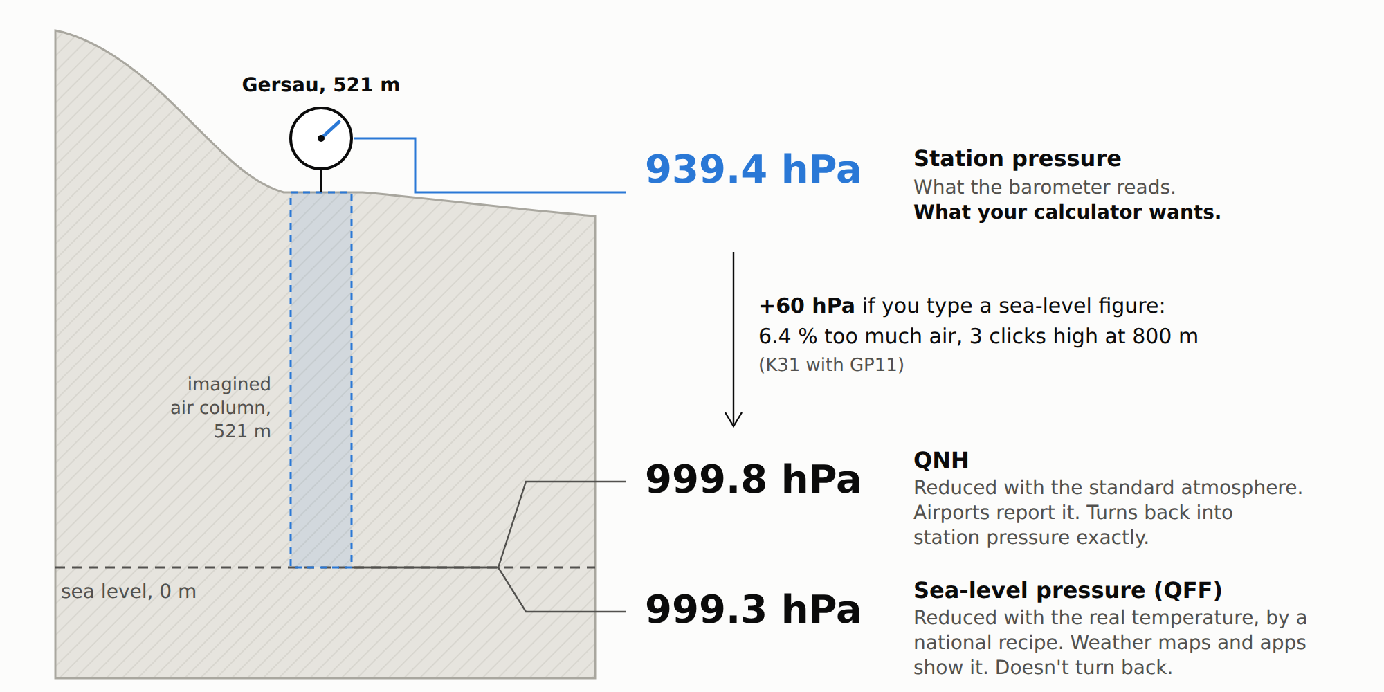
One barometer, three numbers: Gersau on Lake Lucerne, 15 km from Morgarten and one of the eight stations behind Reto’s numbers, at 11:10 that morning (MeteoSwiss). On a mild day at low altitude the two sea-level figures agree within half a hectopascal; in cold weather and higher up they part, and only QNH can be turned back exactly.
Gersau is the gentle case. At 521 m, typing a sea-level figure gives your calculator 6 % too much air, 0.3 mrad high at 800 m. Zermatt, 1638 m, at the same hour: station pressure 820.5 hPa, QNH 1000.7 hPa. Type the sea-level figure there and the air is 22 % too dense, 0.9 mrad high at 800 m (75 cm) and 1.9 mrad at 1000 m. Truing that away takes a BC of 0.334 instead of 0.274.
So the app takes station pressure where it can get it and QNH where it can’t, and converts QNH back exactly. Sea-level pressure it never touches; those stations still contribute temperature and humidity. The smaller traps, rounded QNH and barometers whose listed height is wrong, are dealt with too (A.2).
I did try the shortcut of treating a station’s sea-level pressure as if it were QNH. It made the density error worse than using no pressure from those stations at all, by 2.8 % worldwide and by 7 % at stations above 1500 m. Real station pressure from the same stations made it 2.3 % better.
My advice for any weather source, then: if a pressure isn’t labelled as station pressure or QNH, assume it is sea level and leave it alone.
5. Your height: the number only you can supply
Every station value has to be moved to your height, and pressure changes by about 0.12 hPa per metre near sea level (0.10 at 1500 m). So the height you give the app matters as much as anything the weather services send:
- height read off a topographic map (±1–2 m): ±0.1–0.2 hPa, nothing;
- phone GPS (±5–20 m): ±0.6–2.4 hPa, often the largest pressure error in the whole chain. With 10 m of GPS error, the app’s typical pressure error goes from about 0.8 to 1.5 hPa.
Then there’s the geoid. A browser reports GPS height above a mathematical ellipsoid, not above sea level, and says so in the W3C Geolocation specification, which nobody reads. The difference is the geoid height, and it isn’t small: about +50 m in Switzerland, +48 m in Munich, +37 m in Tokyo, −16 m in Denver, −27 m in Austin, and −99 m in Colombo, Sri Lanka (computed with the geoid model built into the app). Left uncorrected, 50 m is 6 hPa, 0.65 % in density, 0.06 mrad with GP11 at 1000 m, as large as the app’s entire typical error (§16).
The app handles both. A height you type always wins. GPS is averaged over 45 seconds and corrected with a built-in geoid model, which takes the geoid error from 30.6 m typical to about 1.1 m. A map still beats all of that, so type the firing-point height if you can.
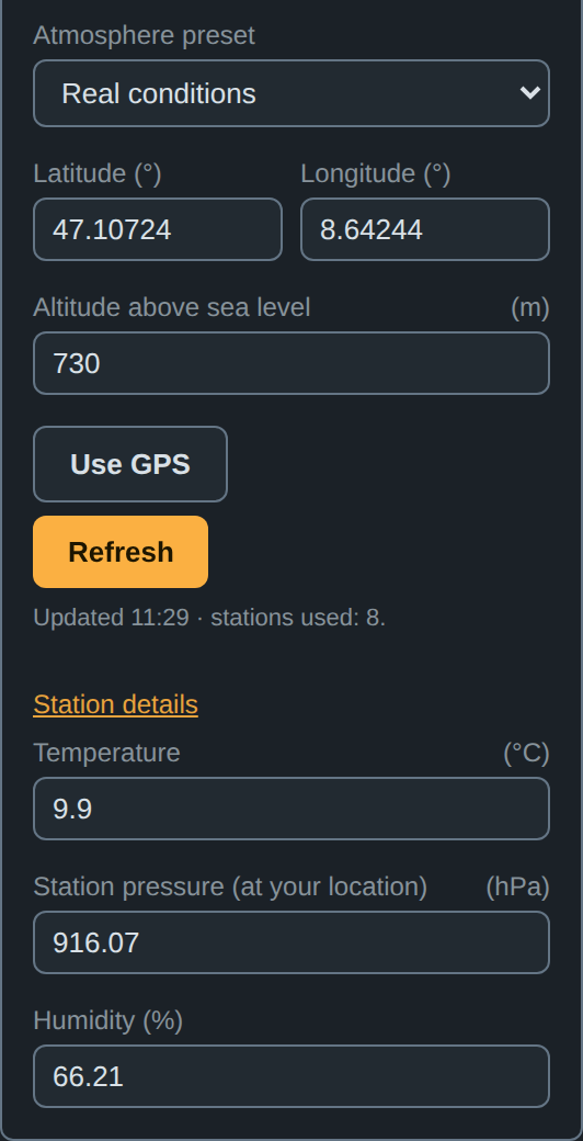
Position, height and the result: 9.9 °C, 916.07 hPa station pressure, 66 % humidity at 730 m, from 8 stations.
6. The stations are not at your height
At Morgarten that morning the eight stations reported anything from 895.9 hPa (Einsiedeln, 911 m) to 943.1 hPa (Wädenswil, 485 m). Taken as they come they’re useless, and even the temperature is off by about two thirds of a degree for every 100 m of height.
So everything gets moved to your height first. Temperature goes with the standard lapse rate, 0.65 °C colder per 100 m. Pressure is moved with the station’s own temperature rather than a textbook one. Humidity I left alone; every cleverer variant I tried was no better (§14).
The lapse rate alone is worth a lot. Without it, the Alpine temperature errors were 13.5 °C where stations stood more than 600 m above or below the target; with it, 5.5 °C. Using the station’s own temperature cut the pressure error by 15 to 45 % in hilly and mountain settings. In density that’s only 1 to 4 %, because temperature dominates. At Morgarten the eight pressures, moved to 730 m, agreed within 1.6 hPa.
7. Nearest is not best
The closest station on the map can be the worst choice, and every “nearest station” weather app makes this mistake. A station on a ridge above you measures different air. Even its QNH can be several hectopascals off the valley’s, because it’s computed through an imaginary column of standard air that doesn’t exist. And a single station, however good, measures its own spot and its own noise.
So the app doesn’t pick a station. It picks up to 8 within 150 km, and then it argues with them (§8, §9). It ranks them by an effective distance in which 100 m of height difference counts like 20 km.
Why should height count as distance at all? §6 moves every station to your height, but with a textbook rule, and the real air between a station and you rarely reads textbooks. On a clear morning the valley floor sits in a cold pool while the slope above is already in the sun. Under an inversion it’s warmer higher up. Föhn does its own thing entirely. The farther a value has to be moved up or down, the more of this it misses, so height difference behaves like distance: the bigger it is, the less the station’s air is yours. A thermometer 3 km away and 60 m above you is a better witness than one 13 km away and 245 m below, and both beat one on a ridge 2 km away and 1000 m up.
The two are combined the way a map combines east and north, as the two sides of a right-angled triangle:
with the distance on the map and the height difference, so 1 m up or down counts like 200 m across, and 100 m like 20 km. Because the two add as squares, whichever is larger dominates. A station 20 km away and 10 m higher is still 20 km away; one 1 km away and 300 m higher is 60 km away. At Morgarten:
| Station | On the map | Height difference | Effective distance |
|---|---|---|---|
| Sattel | 2.9 km | +60 m | 12.4 km |
| Wädenswil | 12.9 km | −245 m | 50.7 km |
| Schüpfheim | 51 km | nearly none | 51 km |
Wädenswil is four times closer than Schüpfheim on the map and ends up level with it. My favourite case is Sion airport, down in the Rhône valley at 482 m. By map distance its nearest neighbour is Plateau Rosa, 3488 m up on the ridge above Zermatt, and using it would cost 6.9 hPa and 6.3 °C of typical error. By effective distance Plateau Rosa is about 600 km away, behind every station in the valley, which is where it belongs.
The effective distance is used wherever the app asks “how close?”. It picks the 8 stations. It sets how much say each one gets, and in the layout weighting of §9 it also decides how alike two stations are, so that two neighbours on the map, one in the valley and one on the slope above it, count as two opinions rather than one. And it decides when the app gives up on that layout weighting (§9). If the app has no height for you, it can only rank by map distance.
The factor of 200 came out of the test of §2 (A.5), not out of my head. The optimum is flat, and anything from 100 to 400 does about as well. What matters is that height counts at all. Worldwide the gain looks small, because most stations in the test stand on flat ground where neighbours share a height and the factor has nothing to do. In the hills and the mountains it decides who gets heard.
Averaging itself was never worse than the nearest station, in any distance band, not even with the nearest under 5 km away. I tried a “close enough, just use that one” switch; it changed nothing, so it’s gone. Shrinking the search radius to 100 or 75 km made things 3 to 5 % worse, so distant stations still help. Against the nearest airport, the finished app takes a sixth off the error even right next to the airport, and nearly a third from 10 to 80 km (§16).
8. Some stations are simply wrong
Meet Richards-Gebaur, near Kansas City (KGVW). It spent all of 2025 convinced it was somewhere warmer: 3 to 15 °C too warm, all year long. At midnight on New Year’s Day it reported 19 °C. The airport 15 km away said 0 °C. Picked as the nearest station for another airport nearby, it handed that one a typical temperature error of 10 °C.
So once all values are at your height, anything far from the group’s median gets thrown out before averaging. How far is “far” depends on how much the stations normally disagree: loose in the mountains, tight on the plains. A fixed tight threshold threw out good mountain data, and no check at all let KGVW through. Dropped stations stay in the table, struck out, with the reason, so you can see who got voted off.
Worldwide the check changes nothing on average, and it shouldn’t; most stations are fine. Where it matters, it matters a lot. In the US Midwest it took the error from 0.479 to 0.455 %, thanks to KGVW.
9. Stations come in crowds
Stations are not independent votes. Three stations around one airport are one opinion said three times. A station hiding behind a nearer one in the same direction adds little; the lone one on the other side of you adds a lot. Weighting by distance alone ignores all of that.
So the app weighs the stations by the distances between them as well as to you. The method is called kriging, which sounds like a Swiss pastry. It’s actually named after Danie Krige, a South African mining engineer who wanted to know where the gold was. Same problem, really: a few holes in the ground, and a guess about the bits in between. Nearer stations still count more, but a crowd has to share its weight and the far side gets its say. Take three stations 20 km east of you and one 23 km west. By distance alone the eastern three get 77 % of the say. With the layout taken into account they get 59 %, and the western one 41 % instead of 23 %.
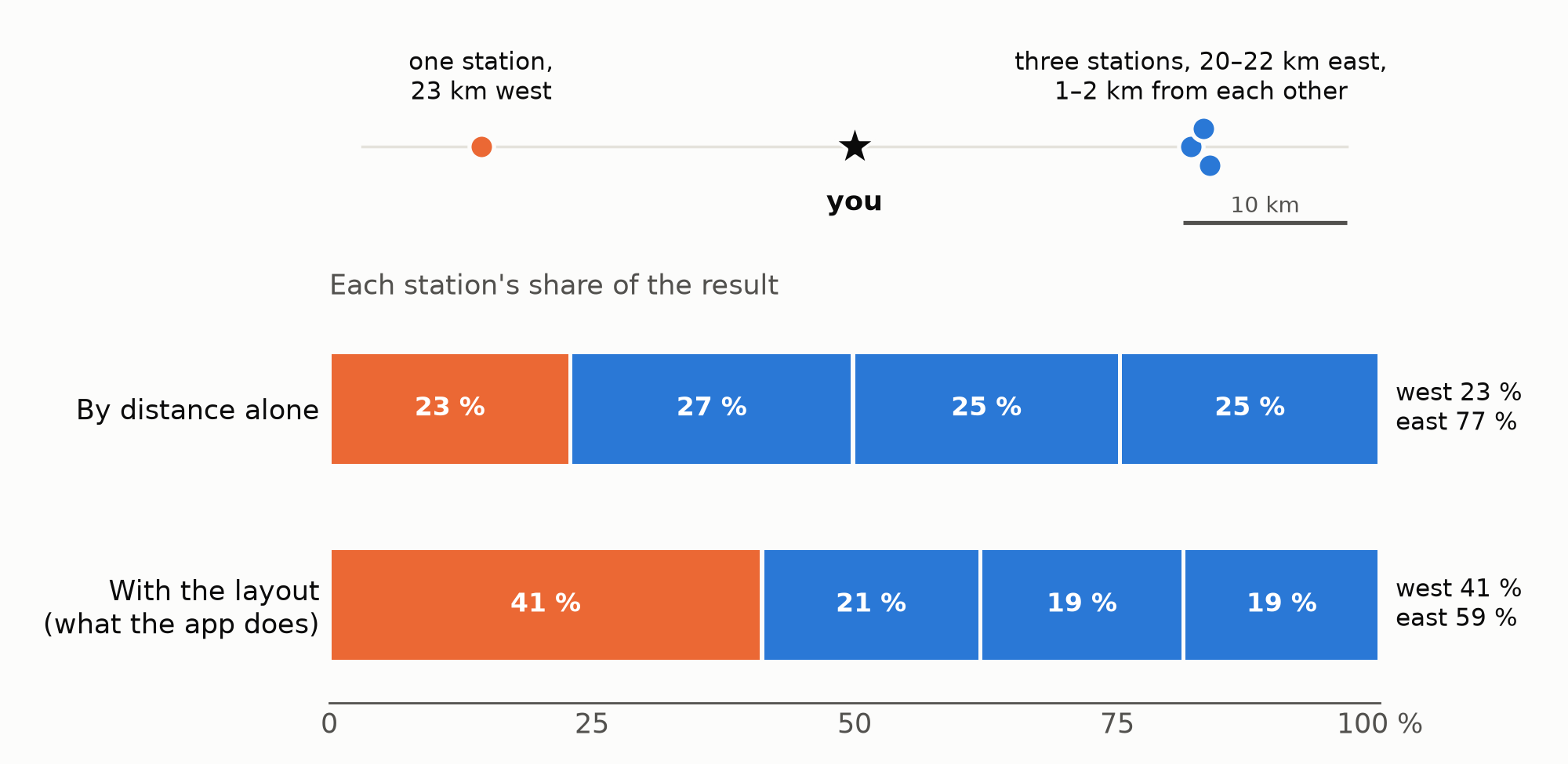
All four stations at your height. If the east reads about 14 °C and the west 10 °C, the result is 13.1 °C by distance alone and 12.4 °C with the layout. Computed with the app’s own combination code.
Kriging has a weak spot of its own. Where even the nearest station is far away, the layout has nothing to offer, and in Peru it once made the estimate 10 to 14 % worse. So beyond about 100 km (effective distance) to the nearest station, the app falls back to plain distance weighting, and Peru is back to even.
Everywhere else it pays: −2.3 % on the density error worldwide, about −3 % where the national networks are in, and −5 % above 1000 m in Austria. On 2024, which played no part in choosing the settings, −2.4 %.
10. The reports are old
Reports are anything from a few minutes to over an hour old when you see them, and temperature moves fastest after sunrise and before sunset, which is exactly when most of us are at the range. On a clear November morning at Morgarten, one hour left uncorrected is 1.7 °C, 0.6 % in air density.
My first idea was the obvious one: draw a line through the last two reports and extend it to now. It made things 15 % worse than doing nothing. Reports come rounded to whole degrees, and a line through two rounded numbers mostly extrapolates the rounding.
What works is the expected daily temperature curve, computed from the sun’s position (time, date, latitude). The app slides each report along that curve from its observation time to now. No extra data, no extra requests. Humidity follows along, same moisture at the new temperature.
For a single station that takes 17 % off the temperature error, on 2024 as well as 2025. Inside the combination of stations it’s 4 %.
11. Clouds change the day
The curve of §10 is an average over all skies. That makes it too small for a clear day and too large for an overcast one. A clear morning warms faster, and clouds cut the day’s temperature swing by a quarter to a half (Dai, Trenberth & Karl 1999). The catch is that most stations don’t report clouds at all.
Airports do. So the app scales the time correction by the cloud cover in the airport reports, and every other station borrows the cover from the airports nearby. I calibrated the correction on airport reports, so that’s all it uses. Other services count cloud differently, and every attempt to convert their figures did worse than simply borrowing (A.9).
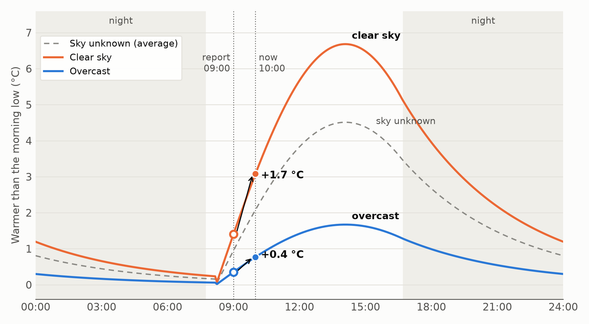
The curve the app uses at Morgarten on 18 November: the sun rises at about 07:40, the low comes half an hour later, the peak shortly after 14:00. The clear-sky hour from 09:00 to 10:00 of §10 (1.7 °C) shrinks to 0.4 °C under overcast, and is 1.1 °C when the sky is unknown.
Overall that’s only −0.5 %. But mornings gain 1.5 % and overcast mornings about 3 %, and for a single station brought forward it’s −6 % in the mornings and −13 % on overcast ones. It hardly ever hurt; only 0.2 % of the stations got more than 5 % worse. The borrowing is what makes it work in the Alps, where only about a fifth of the reports carry their own cover. Without it, the Alps gained nothing.
12. Airports are not where you shoot
Airports sit low and flat. Firing points often don’t. Switzerland has about 12 airports reporting weather and about 158 MeteoSwiss stations; Austria about 6 and 285.
So the app also takes the official non-airport stations: the national networks where they publish open data, and in the US the road-weather and fire-weather stations. This was the biggest single win in this post: 10 % better at airports, 25 to 30 % better everywhere else, and 43 % better above 1000 m. In the American West the road-weather and fire-weather stations took 30 % off away from the airports. And the gain comes from sheer numbers. Rounded to airport precision, the national stations gave almost the same result.
At Morgarten, none of the eight contributors is an airport. The airports only lend their cloud cover.
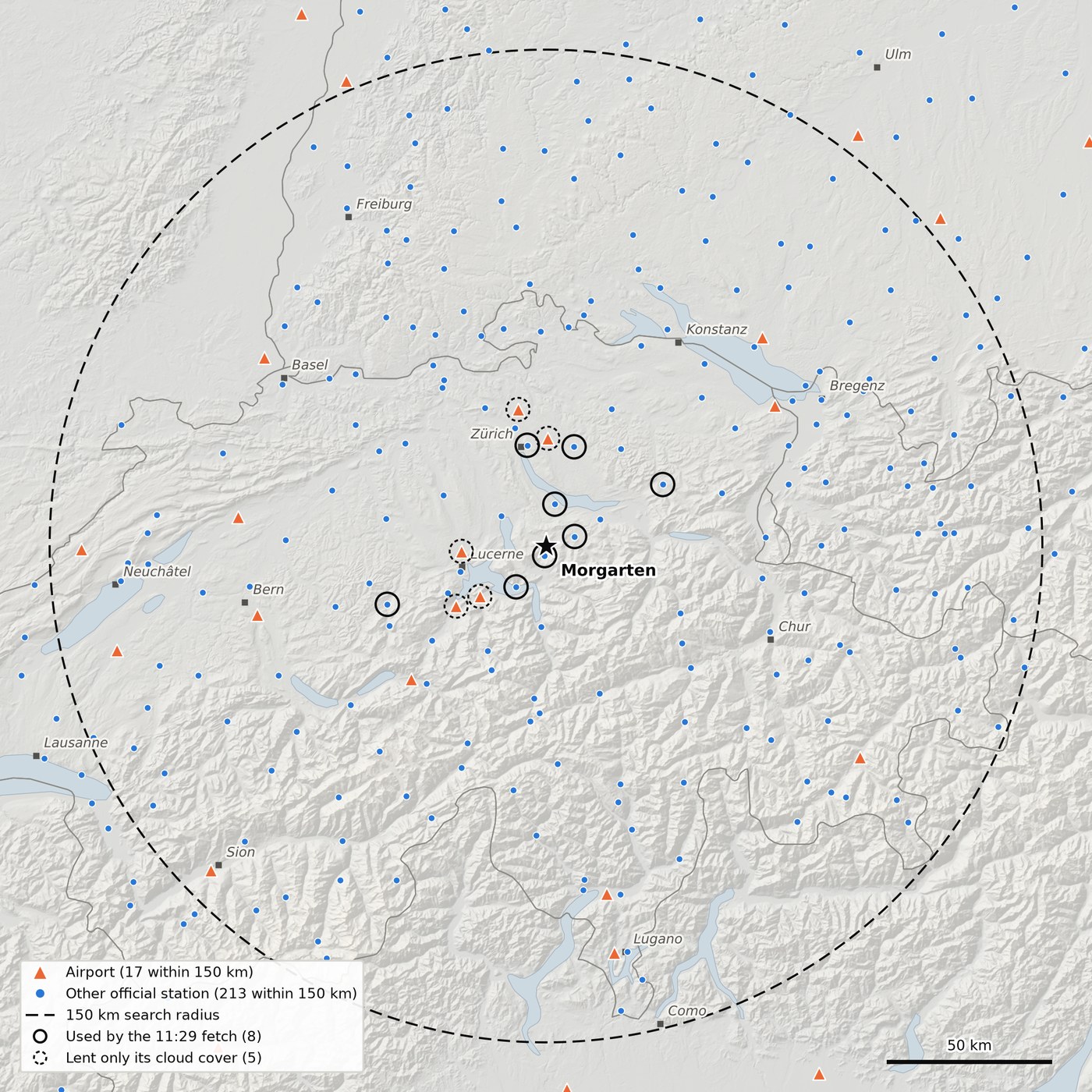
Everything that reported a temperature to the app’s sources at about 13:10 on 18 November 2026: within 150 km of Morgarten, 17 airports and 213 other official stations. Rings: the eight stations the 11:29 fetch actually combined, all MeteoSwiss and all within 51 km; dashed rings: the five airports that only lent their cloud cover. Of 230 candidates, the nearest few at about your height do the work. The airports sit in the lowlands and the big valleys; the mountains belong to the national networks. Across the border in France and Italy, where the app doesn’t use a national network (yet), it is airports and a thin international network only.
13. A number you can’t check is a number you can’t trust
A single figure on a screen tells you nothing about where it came from. So the app shows its work. The station table lists every contributor: distance, height difference, effective distance, age, correction, value at your height and weight.
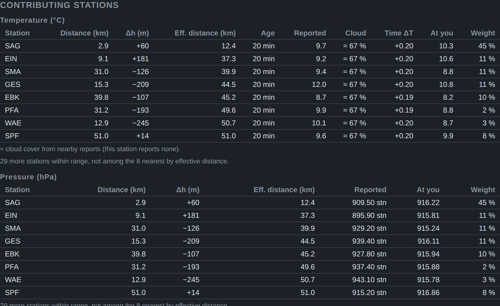
Sattel carries 45 % of the say, Wädenswil only 3 %, Schüpfheim 8 % (their effective distances are in §7). The same table can show a station at 0 %, screened by a nearer one in the same direction; it stays listed.
A glance tells you whether the main contributors are near your height and fresh, or far away on the other side of a ridge (§19). It won’t move the error statistics, but it tells you when to trust the number less.
The app also tries to be a polite guest. The services behind it are mostly public, one is a university, one is a single person’s project, and none of them owes us anything. So it never refreshes on its own, and asks only when a new report can exist.
14. My graveyard of clever ideas
Each of these looked brilliant on paper and lost on data, measured worldwide on a year of hourly reports. I’m listing them partly as a public service and partly because I’m still a bit annoyed.
- Fitting the temperature-height slope to the nearby stations instead of using the textbook one. It gained 0.5 % overall and made a few plateau and mountain sites 20–35 % worse. Not worth it.
- Trusting fresh reports more than older ones. No change at all: once §10 has brought a report forward to now, its age hardly matters.
- Correcting each station’s habitual warm or cold bias. This made things 2 to 5 % worse, and it’s the one with a lesson. A station that is always a bit colder than its neighbours is usually not broken. It lives in a cold spot. So might you.
- Cleverer humidity profiles in height (constant dew point, constant mixing ratio, Hann’s profile). Less than half a percent either way, and one of them put the humidity 5 points too high in the mountains.
15. The whole thing on one page
| Problem | What the app does | What it bought (density error unless stated) |
|---|---|---|
| Model output and citizen sensors | Official measurements only | the starting line |
| Three pressures with one name | Station pressure, then QNH; never sea level | sea level as QNH: +2.8 % (+7 % above 1500 m); station pressure: −2.3 % |
| GPS height above the ellipsoid | Geoid model; typed height wins | height error 30.6 → 1.1 m typical |
| Stations at other heights | Lapse rate; pressure with the station’s own temperature | Alpine temperature 13.5 → 5.5 °C; pressure −15 to −45 % |
| Nearest is not best | Up to 8 stations, height counts as distance | never worse than the nearest, at any distance |
| Broken stations | Buddy check | US Midwest 0.479 → 0.455 % |
| Stations in crowds | Kriging, with a fallback beyond 100 km | −2.3 % worldwide, −5 % above 1000 m in Austria |
| Old reports | Daily temperature curve | temperature −17 % single station, −4 % combined |
| Clouds | Cloud factor, borrowed from airports | −1.5 % mornings, −3 % overcast mornings |
| Airports in the lowlands | National networks | −25 to −30 % away from airports, −43 % above 1000 m |
| All of it together | nearest airport 0.84 % → 0.60 % |
Part III: How good is it
16. The scorecard
The test of §2, 2025, with come-up errors in mrad for K31 + GP11 as in §1:
| Median | Typical (RMS) | 95 % of cases within | 99 % within | |
|---|---|---|---|---|
| Temperature | 0.8 °C | 1.7 °C | 3.4 °C | 5.8 °C |
| Pressure | 0.4 hPa | 0.8 hPa | 1.5 hPa | 2.9 hPa |
| Air density | 0.28 % | 0.60 % | 1.23 % | 2.12 % |
| mrad at 800 m | 0.013 | 0.029 | 0.058 | 0.101 |
| mrad at 1000 m | 0.027 | 0.057 | 0.116 | 0.201 |
Half the time the weather costs you less than 0.013 mrad at 800 m, about a centimetre. One time in a hundred it costs you 0.1 mrad (8 cm) or more.
Against the nearest airport alone: density 0.84 → 0.60 %, temperature 2.26 → 1.65 °C, pressure 1.46 → 0.81 hPa. Away from airports, at the other official stations, 1.04 → 0.63 %. Better everywhere I looked, every continent and every season. Most of all in the mountains, which is where I mostly shoot anyway: above 1500 m, 1.53 → 0.99 %.
Site by site, the app beats the nearest airport by more than 5 % at 88 % of the sites and is more than 20 % worse at 1.5 %. The same test on 2024, which played no part in choosing any setting, gives 0.60 % again.
The error grows with the distance to the nearest airport:
| Nearest airport | Nearest airport alone | The app | The app, mrad at 1000 m |
|---|---|---|---|
| 0–5 km | 0.51 % | 0.42 % | 0.039 |
| 5–10 km | 0.56 % | 0.45 % | 0.042 |
| 10–20 km | 0.78 % | 0.57 % | 0.053 |
| 20–30 km | 0.73 % | 0.51 % | 0.048 |
| 30–50 km | 0.79 % | 0.55 % | 0.051 |
| 50–80 km | 0.93 % | 0.66 % | 0.062 |
| 80–150 km | 1.09 % | 0.84 % | 0.079 |
Even next to an airport, averaging takes a sixth off; from 10 to 80 km, nearly a third. Between 10 and 50 km the distance hardly matters.
The farther the stations, the more you’d want your own meter.
17. Versus a Kestrel
A word first: I am in no way associated with Kestrel. I use their meters as the example because they are common on firing lines and their specifications are published; other pocket weather meters on the market give very comparable precision, and what follows applies to them just as well.
Daytime figures, with Kestrel’s specs read as 95 % limits:
| Air density, typical | Error at 1000 m, typical | The same, on target | |
|---|---|---|---|
| Kestrel 5-series, in shade with airflow | 0.12 % | 0.011 mrad | 1.1 cm |
| Kestrel pocket meter, in shade with airflow | 0.2 % | 0.019 mrad | 1.9 cm |
| Either, in direct sun or still air | 0.4–0.75 % | 0.04–0.07 mrad | 4–7 cm |
| The app, daytime (10:00–16:00) | 0.57 % | 0.053 mrad | 5.3 cm |
| Nearest airport alone, all hours | 0.84 % | 0.079 mrad | 7.9 cm |
In absolute terms the whole contest at 1000 m is about 0.04 mrad, 4 cm on target, between a shaded 5-series and the app.
In the shade with air moving over it, the 5-series is about 4 to 5 times better than the app, the pocket models about 3 times. Almost all of that difference is temperature. The meter knows your spot. The stations know the neighbourhood, which is a different thing, and on a sunny slope a very different thing.
Leave it on the mat in the sun, though, and it’s measuring the mat. In direct sun or still air the sensor warms up by a degree or two (my estimate, not Kestrel’s figure; both Kestrel documents ask for shade and airflow), and then the app is about as good.
Pressure is a tie: about 0.75 hPa for the meter, 0.7–0.9 hPa for the app. So the app is a free check of your meter’s barometer. Kestrel gives the pocket meters a typical drift of −1 hPa per year.
So shade the meter, keep air moving over it, and give it a few minutes. A Kestrel in your pocket is worth eight weather stations, as long as it isn’t in your pocket.
18. What it can’t do
- Calm, clear nights in hollows and on ridges: cold air pools in one and not on the other, 4–5 °C apart.
- Inversions and föhn.
- Broken-cloud days: the reports say how much of the sky is covered, not when the sun comes through. The cloud allowance makes these hours slightly worse (+0.4 %).
- Coast against inland: the marine layer, the sea breeze. There the nearest coastal station is right and the average is wrong. About 4 % of sites do worse with averaging than with their nearest station, mostly these.
- Mountains far from any station.
- Countries without open national networks, much of Asia and Africa: airports only.
- The US: the non-airport stations bring temperature and humidity but no pressure. And they report temperature in whole degrees Fahrenheit, a degree about half the size of a real one and still not fine enough to skip rounding.
- Your exact spot. Stations measure in a white louvred box 2 m above short grass. Your firing point may be sun-heated gravel, or a gully that hasn’t seen the sun since October.
19. Field checklist
- Type your height from a map. Use GPS only if you must.
- In any other weather source, ignore forecasts and anything that is, or might be, sea-level pressure.
- Glance at the station table. Are the main contributors near your height, and fresh? If the only stations are far away or on the other side of a ridge, trust the result less.
- On the coast, or on a calm clear night in a hollow, trust it less again.
- If you own a meter: shade it, ventilate it, and check its barometer against the app now and then.
Weather apps live at sea level. You don’t.
Annex: Geek’s delight
For readers who want the formulas behind Part II. You don’t need any of it to use the app. SI units throughout, temperatures in kelvin inside the formulas. The worked numbers are Morgarten’s fetch of 18 November, 11:29 (the station table in §13), and the K31 with GP11 of §1 in standard air at 730 m (10.25 °C, 928.6 hPa, 50 %).
A.1 Density and what moves it
The calculator wants the density of moist air:
with = 287.05 J/(kg·K) and = 461.5 J/(kg·K) the gas constants of dry air and water vapour, the relative humidity and the saturation vapour pressure. In the reference air:
| Change | Where it comes from | |
|---|---|---|
| +1 K | −0.369 % | = −0.353 %; the rest is the extra vapour at the same relative humidity |
| +1 hPa | +0.108 % | |
| +10 % RH | −0.051 % | ; at 30 °C −0.17 %, because doubles about every 11 K |
Dividing the first line by the second gives the 1 K ≈ 3.4 hPa of §1. The come-up is linear in the density error at these sizes: per 1 % of density, GP11 needs 0.021 / 0.047 / 0.094 mrad at 600 / 800 / 1000 m. A calculator that takes the powder temperature from the air temperature adds = 0.8 m/s per K on top, which turns 0.006 / 0.014 / 0.027 mrad per kelvin into 0.020 / 0.035 / 0.059.
The kelvin figures are net of the speed of sound, which rises by about 0.6 m/s per K. The bullet then flies at a lower Mach number, and near Mach 1, where GP11 arrives at 1000 m (Mach 1.06), a lower Mach number means more drag. For 1 K warmer, that puts back 0.004 mrad at 800 m and 0.008 mrad at 1000 m of the 0.017 and 0.034 mrad that the thinner air takes off. The powder term alone is worth 0.022 mrad at 800 m and 0.033 mrad at 1000 m per kelvin.
A.2 Pressures and their inverses
QNH is defined through the standard atmosphere, so it inverts exactly:
with = 1013.25 hPa, = 288.15 K, = 0.0065 K/m and = 9.80665 m/s². The shortcut , which you will find in plenty of code, is exact only when QNH happens to be 1013.25. At Morgarten on 18 November it was 0.2 hPa off; at 1500 m with a QNH of 980 or 1045 hPa, about 1 hPa.
European airports report QNH rounded down to the whole hectopascal. If the remainder is spread evenly, its expectation is 0.5 hPa, so the app adds that. Measured: the pressure bias went from −0.37 to +0.01 hPa. US airports report the same QNH in inches of mercury, to the hundredth: the height of a column of liquid metal, a proud tradition. Ironically, it’s the finer resolution of the two (0.01 inHg is 0.34 hPa), and it needs no such correction.
Sea-level pressure (QFF, MSLP) has no such inverse. Each weather service reduces it with its own recipe: the current temperature, a 12-hour mean, special rules for high stations. Treated as QNH, it made the density error 2.8 % worse than no pressure from those stations at all, 7.2 % worse at targets above 1500 m. Undoing the reduction with the station’s own temperature got back only 0.4 %; the same stations’ real station pressure gave 2.3 %.
Station pressure needs the barometer’s height, which is not always the station’s. The app checks it: below 800 m, the height implied by a station’s pressure and its QNH or QFF must match the listed one within a few tens of metres. Zürich/Fluntern moved 48 m uphill in June 2026, and one station list still had the old height; its perfectly good pressure arrived 6 hPa low, and the buddy check (A.6) threw it out. Innsbruck Universität’s pressure implies a barometer 30 m above its listed height; the app leaves it out.
A.3 Moving values in height
Temperature moves with the standard lapse rate, . Pressure moves with the hypsometric equation and the station’s own temperature:
A QNH is first taken to station level with A.2, which is exact, and then moved with this. Against the standard-atmosphere version, the pressure error fell by 15 to 45 % in hilly and mountain settings, the density error only by 1 to 4 %, and nothing in the flat. The density gain is smaller because in daytime the pressure error and the temperature error become correlated: both now rest on the same sun-heated 2 m temperature.
Relative humidity is left as reported in height. Constant dew point, constant mixing ratio and Hann’s vapour-pressure profile all changed the density error by less than half a percent; the constant mixing ratio put the humidity 5 points too high in the mountains. In time, the vapour pressure is held and the humidity recomputed for the corrected temperature: .
At Morgarten, the eight station pressures ran from 895.9 hPa (Einsiedeln, 911 m) to 943.1 hPa (Wädenswil, 485 m). At 730 m they ran from 915.2 to 916.9 hPa.
A.4 Height and the geoid
GPS gives the height above the WGS84 ellipsoid; maps give the height above the geoid, roughly mean sea level; . The app carries the geoid height as a spherical-harmonic series to degree 72 fitted to EGM2008: 5329 coefficients, 21 KB, about 1.1 m RMS worldwide and 20 m at the very worst spot. The trade-off, measured against a global grid:
| Model | Size | RMS | Worst |
|---|---|---|---|
| no correction | 0 | 30.6 m | 107 m |
| degree 18 | 1.4 KB | 2.7 m | 25 m |
| degree 36 | 5.3 KB | 1.8 m | 22 m |
| degree 72 | 21 KB | 1.1 m | 19 m |
| degree 180 | 128 KB | 0.4 m | 6 m |
GPS heights are averaged over 45 seconds. Pressure falls by about 0.12 hPa per metre, so 10 m of GPS error is 1.2 hPa, and the app’s typical pressure error of 0.8 hPa becomes hPa.
A.5 Effective distance and selection
so 100 m of height difference counts like 20 km. Sattel, 2.9 km away and 60 m higher, is 12.4 km away by this measure; Wädenswil, 12.9 km away and 245 m lower, is 50.7 km; Schüpfheim, 51 km away at nearly your height, stays at 51 km. Per quantity, the 8 nearest by within 150 km take part, with reports up to 90 minutes old. The optimum is flat (density RMS worldwide, at an earlier stage of the method):
| Setting | Values tried (density RMS) |
|---|---|
| 0: 0.650 % · 50: 0.645 · 100: 0.641 · 200: 0.639 · 400: 0.641 | |
| stations | 4: 0.648 · 8: 0.641 · 12: 0.643 · 20: 0.648 |
| search radius | 75 km: 0.672 · 100 km: 0.661 · 150 km: 0.641 |
| nearest only, if within 5 km | 0.641, identical to always combining |
Distant stations still help, and a “close enough” switch buys nothing.
A.6 The buddy check
With at least three values at your height, the app takes their median and median absolute deviation (MAD), and drops any value with
estimates the standard deviation of well-behaved data without letting the outlier inflate it. Humidity is not checked. On three regional test sets, at an earlier stage of the method (density RMS):
| Check | Alps | US Midwest | Norway |
|---|---|---|---|
| none | 0.766 % | 0.478 % | 0.956 % |
| fixed 5 K / 3 hPa | 0.800 % | 0.460 % | 0.965 % |
| scaled with the MAD | 0.780 % | 0.452 % | 0.959 % |
A fixed tight threshold throws out good mountain data; no check lets KGVW through. The scaled one is never the worst anywhere.
A.7 Weights: kriging, with a fallback
Ordinary kriging picks the weights that minimise the expected error for a given covariance between stations, under :
where is the effective distance between stations and (A.5, with their height difference), = 200 km and the nugget = 0.1, the share of a station’s variation that no other station shares. is the Lagrange multiplier. Negative weights are set to zero and the rest scaled back to 100 %, which keeps every weight displayable in the station table. If even the nearest contributor is more than 100 km away (effective), the app uses instead.
At Morgarten (weights in %, as displayed):
| SAG | EIN | SMA | GES | EBK | PFA | WAE | SPF | |
|---|---|---|---|---|---|---|---|---|
| , km | 12.4 | 37.3 | 39.9 | 44.5 | 45.2 | 49.6 | 50.7 | 51.0 |
| by distance alone | 50 | 9 | 9 | 7 | 7 | 6 | 6 | 6 |
| kriging | 45 | 11 | 11 | 11 | 10 | 2 | 3 | 8 |
Pfäffikon and Wädenswil lie on the Zürich side, behind Fluntern, and lose most of their say; Schüpfheim, alone to the west, gains. The textbook vector of the figure in §9 (three stations east, one west) goes 77/23 → 59/41 %.
Results: −2.3 % worldwide in 2025, −2.4 % in 2024, −1.8 to −3.1 % with the national networks (Greenland and the Faroes: nothing). Without the 100 km fallback, Peru got 9.5 % worse in 2025 and 13.8 % in 2024; with it, Peru is back to even. The simpler fixes that kriging contains each gave about half as much: Shepard’s (1968) direction factor −0.9 %, at most two stations per quadrant −1.3 %, de-clustering −1.0 %. For the theory, any geostatistics text, e.g. Cressie (1993).
A.8 Bringing reports forward: the daily curve
Each temperature report is moved from its observation time to now along an expected daily curve. The curve needs nothing but the station’s position, the date and the clock.
The sun first. With the day of the year, the declination is (Cooper 1969). The day length in hours is
with the latitude. In local solar time, the sun rises at and sets at . Solar time is UTC plus 4 minutes per degree of east longitude plus the equation of time, minutes, with .
Then the shape, after Parton & Logan (1981): a sine by day, an exponential decay by night.
where is the time since sunset. The published constants are = 1.86 h, = 2.2 and = −0.17 h, fitted at one site in Colorado. Refitted on a year of hourly reports worldwide, they became = 1.4 h, = 3.0 and = +0.5 h: the low comes half an hour after sunrise. Fitting separate shapes per latitude band added nothing.
The size of the swing is , the second factor being the sine of the sun’s height at noon. comes from a table, interpolated in latitude:
| Latitude | 5° | 15° | 26° | 35–44° | 54° | 64° | 72° |
|---|---|---|---|---|---|---|---|
| 6.8 K | 8.0 K | 9.5 K | 12.4 K | 9.5 K | 9.4 K | 6.3 K |
It peaks in the dry continental mid-latitudes and falls off toward the humid tropics on one side and the cloudy, maritime north on the other, so no straight line in latitude fits it. The correction is then
with the cloud factor of A.9. Humidity follows the new temperature at constant vapour pressure (A.3).
At Morgarten on 18 November: = −19.8°, the sun stands 23° high at noon, = 11.5 K and = 4.5 K. The day is 8.9 h long, the sun rises at about 07:40, the low comes at 08:15 and the peak at 14:05, all in local time. Sattel’s 11:10 report, used at 11:29, moves along the curve from 0.706 to 0.766: +0.27 K before clouds. With the 67 % cover borrowed from the airports, = 0.74, which gives the +0.20 K in the station table.
Tested on its own, against simply using the last report: −17.5 % in temperature error when fitted on 2025 and tested on 2024, and −18.3 / −18.0 % when fitted on one half of the stations and tested on the other. By latitude, the gain is 17 to 19 % up to 50°, 9.5 % at 50–60°, 5.5 % at 60–70° and about 1 % beyond, where the sun barely moves in winter. Inside the combination of stations it takes 4.5 % off the temperature error. A version that learns each station’s own daily rhythm from its last 14 days does barely better (−18 % single-station, −4.6 % combined) and would need a history the app can’t collect from a phone that is used now and then at changing places.
A straight line through the last two reports fails because the reports are rounded and noisy, and the line amplifies both. It is 15 % worse than doing nothing, and 32 % worse where whole-degree reports come every 30 minutes. Damped to a quarter of its slope, it gets back to about neutral.
A.9 The cloud factor
The table of was fitted on all skies, so it is too small for a clear day and too large for an overcast one. The app scales the correction by the cloud cover (fraction of the sky):
is the mean cover of a year of airport reports worldwide, so on average = 1 and the fit of A.8 stays intact. A clear sky gives = 1.48, overcast 0.37, an unknown sky 1. Normalising matters: damping alone () helps overcast hours but makes clear mornings 0.7 % worse, because then nothing stretches the too-small clear-sky swing. The factor applies at night too, because clouds also slow the evening and night cooling; a daytime-only version did worse.
The cover comes from the airport reports, as the largest layer: FEW 2/8, SCT 4/8, BKN 7/8, OVC and vertical visibility 8/8; CAVOK, NSC, NCD, CLR and SKC count as clear. Synoptic and national stations send no cover the app can use. They borrow the regional cover: the mean of the airport covers within 100 km of you, weighted by , with the airport’s distance from you. Worldwide, 79 % of the contributing reports carry their own cover and 96 % have one after borrowing. In the Alps only about 20 % carry their own, so without borrowing the Alps gained nothing. At Morgarten, the five nearby airports gave 67 %.
The German weather service publishes a total cover for many of its stations, but the app ignores it. At eight German airports, over 66,000 common hours, it averaged 69 % against the airport reports’ 35 %: it counts all cloud up to the cirrus, the airport report only the lower layers. Its 8/8 hours range from clear to overcast in the airport reports. Every conversion I tried (a shift, a shift and shrink, a table per eighth) did worse than borrowing the airports’ cover: at best −0.62 % against −0.66 % in Germany.
Results, density error, against the same method without clouds:
| All hours | Mornings (06–10) | Evenings (16–20) | Night | Overcast mornings | |
|---|---|---|---|---|---|
| combination of stations | −0.5 % | −1.5 % | −0.7 % | −0.1 % | −3.0 % |
| a single station brought forward | −2.0 % | −6.2 % | −12.8 % |
By the sky at the target: clear −0.5 %, overcast −0.8 %, partly cloudy +0.4 %. A cover of 3 to 6 eighths says how much of the sky is covered, not when the sun comes through. Per station, none got more than 20 % worse and 0.2 % more than 5 % worse. The gain is small because the cloud factor can only refine the time correction, which is worth 4.5 % in all; mornings gain most, and that is when most shooting starts. Of the slopes tried (0.25, 0.5, 0.75), 0.75 did best. It gives an overcast sky a quarter of the clear-sky correction, a stronger cut than the 25 to 50 % that Dai, Trenberth & Karl (1999) found for the daily temperature range; the slope was chosen by the errors, not by their figure.
A.10 How it was validated
Leave-one-out on NOAA’s hourly archive (GHCNh): each station in turn plays your phone, is predicted from the others within 150 km, and its own report is the truth. 5404 targets, 3897 airports and 1507 other official stations, 58 million hours in 2025; 2024, which played no part in choosing any setting, as the out-of-sample check. Reports arrive as they would live: airports 5 minutes after observation, synoptic stations on the hour plus the measured publication delay of their country (6 to 21 minutes), nothing older than 90 minutes. Hours where the target itself is more than 15 K or 10 hPa from the median of its 8 nearest neighbours are skipped for every method alike (0.06 % and 0.15 % of hours; without this filter the ranking of the methods is the same). All variants are scored on the same hours. The national networks were validated in the same way, over their own data periods.
What the test can’t see: the truth is a station in a standard screen, mostly on open ground; your height error and the geoid (A.4) come on top; and your own spot is not a station.
What didn’t make it, with the change in density RMS:
| Idea | Effect |
|---|---|
| temperature–height slope fitted to the nearby stations | −0.5 %, but 20–35 % worse at a few plateau and mountain sites |
| fresh reports weighted more than old ones | ±0 % |
| each station’s habitual bias removed | +2 to +5 % |
| a line through the last two reports | +15 % |
| sea-level pressure treated as QNH | +2.8 % |
| smaller search radius (75 / 100 km) | +5 / +3 % |
A.11 The Kestrel arithmetic
Kestrel’s accuracies taken as 95 % limits, so one standard deviation is half the listed figure; the three terms are independent and add in quadrature, with the sensitivities of A.1.
| Temperature | Pressure | Humidity | Density | |
|---|---|---|---|---|
| 5-series: 0.5 °C, 1.5 hPa, 2 % RH listed | 0.25 K → 0.092 % | 0.75 hPa → 0.081 % | 1 % → 0.005 % | 0.12 % |
| pocket meters: 1.0 °C, 1.5 hPa (+1 hPa/year drift), 3 % RH | 0.5 K → 0.18 % | 0.75–1.3 hPa → 0.08–0.14 % | 1.5 % → 0.008 % | 0.20–0.23 % |
| either, sensor 1–2 K warm in the sun | +0.37–0.74 % | 0.4–0.75 % |
The density-altitude figure: in the standard atmosphere near sea level, density falls by ≈ 0.0096 % per metre, so ±226 ft = ±69 m is ±0.66 % in density. The same sheet lists relative air density at ±0.3 %.
Sources
Data:
- Iowa Environmental Mesonet, Iowa State University: airport (METAR) and synoptic (SYNOP) reports, US road-weather and HADS networks. https://mesonet.agron.iastate.edu/
- MeteoSwiss, SwissMetNet open data (CC BY 4.0). https://opendatadocs.meteoswiss.ch/
- GeoSphere Austria, TAWES open data (CC BY 4.0). https://data.hub.geosphere.at
- Deutscher Wetterdienst, via Bright Sky (CC BY 4.0). https://brightsky.dev/
- Danish Meteorological Institute, open data (CC BY 4.0). https://opendataapi.dmi.dk
- Environment and Climate Change Canada, NAV CANADA and partner networks, MSC GeoMet. https://api.weather.gc.ca
- Validation archive: NOAA NCEI, Global Historical Climatology Network hourly (GHCNh), 2024 and 2025. https://www.ncei.noaa.gov/oa/global-historical-climatology-network/hourly/
Map:
- Relief: Copernicus DEM GLO-90, © DLR e.V. 2010–2014 and © Airbus Defence and Space GmbH 2014–2018, provided under COPERNICUS by the European Union and ESA; all rights reserved. https://registry.opendata.aws/copernicus-dem/
- Borders and lakes: Natural Earth (public domain). https://www.naturalearthdata.com/
- Stations: the station lists and current reports of the sources above, 18 November 2026.
History:
- John of Winterthur (Johannes Vitoduranus), Chronica, ed. F. Baethgen, MGH Scriptores rerum Germanicarum, Nova series 3 (1924). The Latin of the halberd passage as quoted by A. Baschung, “Halberd – the rise of an all-purpose weapon”, Swiss National Museum blog, 24 January 2022. https://blog.nationalmuseum.ch/en/2022/01/the-rise-of-the-all-purpose-weapon-halberd/ The other quotations are my translations of the German in W. Oechsli, Quellenbuch zur Schweizergeschichte (1918), pp. 61–63.
- Historisches Lexikon der Schweiz: Reding, Alois. https://hls-dhs-dss.ch/de/articles/007276/
- Morgartenschiessen. https://morgartenschiessen.ch/
- Swiss Shooting (SSV): Eidgenössisches Feldschiessen. https://www.swissshooting.ch/
Literature and specifications:
- Cooper, P. I. (1969). The absorption of radiation in solar stills. Solar Energy 12, 333–346.
- Dai, A., Trenberth, K. E., Karl, T. R. (1999). Effects of clouds, soil moisture, precipitation, and water vapor on diurnal temperature range. Journal of Climate 12, 2451–2473.
- Cressie, N. A. C. (1993). Statistics for Spatial Data, revised edition. Wiley.
- Parton, W. J., Logan, J. A. (1981). A model for diurnal variation in soil and air temperature. Agricultural Meteorology 23, 205–216.
- Pavlis, N. K., Holmes, S. A., Kenyon, S. C., Factor, J. K. (2012). The development and evaluation of the Earth Gravitational Model 2008 (EGM2008). Journal of Geophysical Research 117, B04406.
- Shepard, D. (1968). A two-dimensional interpolation function for irregularly-spaced data. Proceedings of the 1968 23rd ACM National Conference, 517–524.
- W3C, Geolocation API (altitude above the WGS84 ellipsoid). https://www.w3.org/TR/geolocation/
- ICAO, Annex 3, Meteorological Service for International Air Navigation (QNH rounded down to the whole hectopascal); ICAO Doc 7488, Manual of the ICAO Standard Atmosphere.
- Kestrel Instruments, Product Specifications for Kestrel 5 Series Weather/Environmental Meters (2025). https://kestrelinstruments.com/mwdownloads/download/link/id/21/
- Kestrel, Specifications for Kestrel pocket weather meters. https://kestrelmeters.com/pages/specifications-for-kestrel-pocket-weather-meters